About
Theoretical background
A species response curve typically describes the performance of a species in response to a gradient of a single abiotic environmental factor. These curves often, but not necessarily always, show an upper and lower limit for the persistence of a species and a range of conditions where the species have a good and optimal performance. Thus, a species response curve will typically describe under which conditions a species will be absent or can be present (i.e., referred to as niche width or tolerance), and if the species can be present, which densities the species may reach given the value of that specific environmental setting.
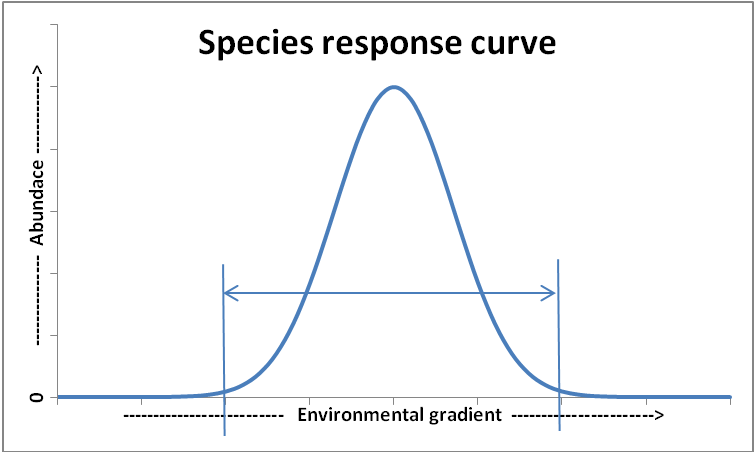
species response curve.
Environmental parameters
In the natural environment, there are of course a range of abiotic environmental factors for which a species will have a species-specific response curve. The actual abundance of a species will be determined by the environmental factor which has the most restricting value on the species response curve (i.e., the limiting factor). As soon as the condition of the limiting factor changes, the abundance of the species will change and stabilise at a new equilibrium. Depending on the species, abundance may be defined as (areal) biomass, (areal) number of individuals, shoot density, leaf density, etc.
In general, the closer an environmental parameter is to the species’ upper or lower tolerance limits, the more stressful this is. Although a single limiting factor may restrict a species occurrence, it is too simple to see all abiotic factors as fully independent. The value of one variable, especially if it is close to a species’ tolerance limit, may also have a limiting effect on the niche width or optimum value of another environmental parameter. E.g. the temperature niche width of seagrasses decreases with reducing light availability, because the energy consumption via respiration is higher at higher temperatures, while the energy production needed to maintain this higher respiration is lower at lower light intensity. Due to these kind of interactions between environmental parameters, the actual species response curve for a specific environmental variable may differ between locations.
Species response and species trajectory curves
The above-described Gaussian shaped species response curve is static in that it does not explicitly address temporal aspects about i) temporal variability in environmental conditions, ii) how long species can tolerate conditions outside the average tolerance limits and iii) the time required for a species to adjust to changing conditions. This makes it difficult to use a species response curve to derive the impact of temporal variability in abiotic conditions on a species performance. Short-term exceedance of average tolerance limits may however occur regularly e.g. due to temporal natural environmental variability. Species can have mechanisms to overcome conditions that exceed their average tolerance limits, but the dynamics of these mechanisms do not necessarily match up with the temporal variability causing the exceedance of average tolerance limits. The impact of exceeding tolerance limits has been related to the intensity, duration and frequency of the occurrence of environmental parameter(s) (e.g., for corals see Newcombe and MacDonald, 1991; McArthur et al., 2002). Therefore, an alternative to describe a species response to an environmental factor, is to plot a species response trajectory curve. A species response trajectory shows species abundance as a function of time under a specific environmental condition. The figure below illustrates this for different stress levels.
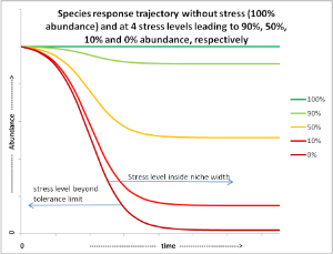
Maintaining a ‘stress’ level corresponding with the environmental parameter value at which the occurrence of a species is optimal (indicated by the dark green 100% line in the figure above) does not lead to changes in abundance relative to t=0. If environmental factors change to a stress level beyond a species’ tolerance limit, this will lead to 0% abundance over time (dark red 0% line in figure above). However, as long as a new stress level does not exceed the species tolerance limit, species abundance will stabilise at a new (equilibrium) level. This new (equilibrium) level may be the result of e.g. increased mortality of individuals, reduced growth rates, reduced reproduction, etc., in response to e.g. reduced resources or physiological limitations. When the stress level at a specific location exceeds the species tolerance level too long, the species will be eventually lost at such a location. Before this point is reached, however, timely stress remediation may prevent species loss. Where (abundance level) and when (response time) this point is reached is difficult to predict and depends on species’ specific resilience. Removing stress not necessarily immediately leads to improvements. A downward trend may continue for some time and could still result in the loss of a species. In general, the closer to its tolerance limits a species persists, the more vulnerable it will be to disturbances.
Combining Graphs
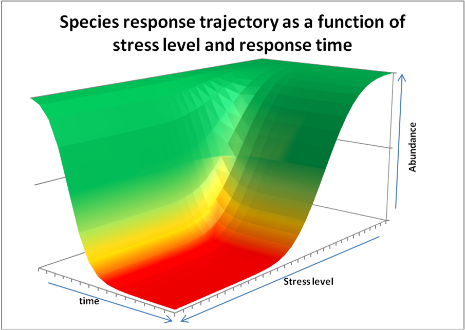
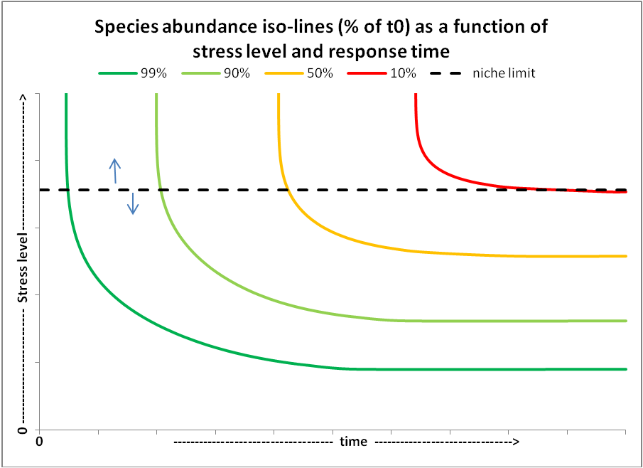
Combining the species response curve shown in the top figure (note: we only show one part of the curve between maximum and zero abundance, by plotting stress level from no stress optimal conditions to stress levels beyond a tolerance limit) and the species response trajectory curves shown in the second figure, results in a 3D representation of how species respond over time to increased stress levels due to changing environmental parameters from optimal at t=0, to the stress level indicated in the figure (see the third figure below). Making a 2D top-view projection of the third figure, results in species abundance iso-lines (in % of t=0 value) from which one can see the resulting abundance (proxy for health status) of a species (colours) as function of stress level and exposure time to that stress level. In case the combination of stress level x exposure time is too high, species cannot persist and will disappear.
abundance as a function of species response
time in relation to stress level, defined as being
exposed to sub-optimal environmental conditions.
The actual shape of the species response trajectory depends on the species-specific capacity to acclimate to the imposed stress and the time needed for such acclimation. In case of seagrasses being exposed to light stress, acclimation might involve an increase in chlorophyll content in their leaves as to increase photosynthetic efficiency in response to light reduction and maintain the abundance (see figure below). However, if such acclimation is insufficient, other aspects may be affected, ultimately reducing species abundance. If, when and how different response mechanisms are activated determines the development of species abundance over time. Changes in abundance could be gradual or very sudden (see Fig. 7 below), or occur in steps, whereby an initial increase in abundance is not impossible. All schematised curves in this section are (seagrass) species specific, meaning that predicting a community response requires combining this knowledge for different (seagrass) species or assuming that all species in the community behave roughly the same. The latter might be acceptable in case little information is available on individual species making up the community.
response based on a measurable stressor adapted from Erftemeijer et al., 2012).
Building with Nature interest
Knowledge about species response time and response trajectory shape in relation to stress level is essential to provide useful information to coastal managers and policy-makers for the assessment of potential damage to ecosystems e.g. dredging operations and coastal infrastructural works and to implement protective measures. Reduced light penetration resulting from poor water quality is among the most significant of impacts threatening seagrass ecosystems worldwide (Waycott et al., 2009). For some activities, such as dredging, protective measures can be put into place to minimise the impact of increased turbidity (suspended sediment) and concurrent light reduction, and manage the consequences for seagrass systems (Erftemeijer and Lewis III, 2007). However, this is often not possible. In those cases, knowledge about the resilience boundaries of seagrass ecosystems in relation to the expected environmental impact is crucial in the planning and design phase of the operation, in order to avoid irreversible damage or loss.
Seagrass response to light limitation: state of the art
In Singapore seagrasses are concentrated around the smaller islands to the south, but there are also sites along the shores of Singapore’s mainland. Most of Singapore’s seagrass meadows are intertidal. Singapore is aware of the need for seagrass protection, monitoring, management, and restoration. The coastal and marine ecosystems of Singapore are however limited and modified by development and the port industry (which is one of the biggest income-earning businesses in the country). For most seagrass species, threshold levels of light reduction are not known, hampering the ability of coastal resource managers to identify impacts and take appropriate measures (Ralph et al., 2007). Seagrasses have the ability to respond to their highly variable light environment and tolerate periods of reduced light availability, balancing photosynthetic (= light dependent) energy production and energy consumption (respiration).
A sequence of possible responses is given in in the figure below (Collier et al., 2011). How the combination of a reduction in light intensity and the duration of such light reduction cause such responses and control the specific nature and magnitude of adaptations is still poorly understood. Moreover, the latter may differ considerably depending on species-specific growth and survival strategies and the specific environmental setting where the plants grow. Physiological responses can take place on timescales of hours to days, whereas timescales of morphological responses may take weeks to months before they become visible. Visible responses on community scale may take weeks to up to a year, depending on the species composition of a community. Pioneer species usually show a faster response compared to climax species.
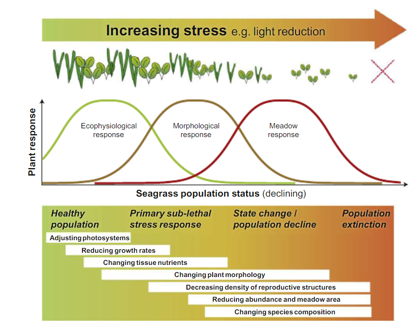
In general, fast growing pioneer species with limited biomass and energy reserves and relatively low respiratory energy demands, typically have lower minimum light requirements compared to slow growing climax species with larger biomass and energy reserves and relatively high respiratory energy demands (ecophysiological response range). Yet, these fast growing pioneer species are more sensitive to light reduction and do not tolerate prolonged periods of low light, while slow growing climax species can tolerate much longer periods of light stress (morphological response range) (Collier et al., 2011). On the other hand, the pioneer species recover much faster from the effects of light reduction when light conditions return to normal, whereas the recovery from loss by climax species usually takes much longer and may not occur at all (meadow response range).