1. Clear and turbid lakes
In general, two types of shallow lakes can be distinguished. One is characterised by high water transparency, dominance of aquatic vegetation, small amounts of nutrients and a diverse fish community. The other type is characterised by turbid water, with no or small amounts of aquatic vegetation, large amounts of nutrients, large seasonal algal blooms and a fish community that is dominated by large benthivorous fish species like bream. Both states can be stable under the same environmental conditions. Under such conditions, larger disturbances may cause the system to shift from one state to the other: a ‘regime shift’. The theory of alternative stable states explains why ecosystems (in general) can have multiple stable states.
Alternative stable states
The following overview of the alternative stable states theory has been provided by Ingrid van de Leemput, PhD candidate at the aquatic ecology and water quality management group of the Wageningen University.
A system may have alternative states, if it has internal positive feedback loops that can amplify the effect of a disturbance. For example, a nutrient pulse in a shallow lake can increase algal biomass temporarily, which results in low water transparency, leading to increased competitive strength of algae over macrophytes. This change will in turn lead to an increased level of sediment disturbance, which lowers the water transparency even more. As a result of this cascade of processes, the system is trapped in a turbid situation even after the nutrient pulse has ceased. Similarly, temporary removal of benthivorous fish species in a turbid lake may trigger a shift to a clear state, through a decreased level of sediment disturbance, higher water transparency, and the growth of aquatic plants. In general, if a system that has multiple stable states is in a certain stable state, it tends to stay there, unless its driving factors exceed a certain threshold and push it to another stable state. Moving from one stable state to another and back may involve ‘hysteresis’, implying that the return to the initial state requires a stronger change of the driving factors than the one that triggered the regime-shift.
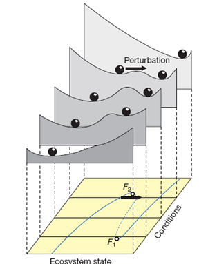
One way to explain the theory of alternative stable states is the ball-in-a-cup analogy (adjacent figure; Scheffer et al., 2001). In this representation the valleys in the stability landscape represent the different stable equilibriums; the hilltops unstable equilibriums .The ball represents the current state of an ecosystem. If the ball is situated in a deep valley, the resilience of that particular system is high, because a small perturbation will not be able to push the system out of its equilibrium. In contrast, if the valley is shallow, ecosystem resilience is low, and the system is more easily shifted by a disturbance. Environmental conditions will alter the shape of the landscape, and thus the resilience of the system. For example, increased nutrient inflow into a shallow lake with clear water will disturb the state of the system. If the nutrient inflow reaches a critical level, the clear water state is not stable anymore, and the system shifts to a turbid stable state. This point is called a ‘tipping point’, and the state shift that occurs at this point is called a ‘critical transition’.
So far virtually all theoretical underpinning of this view of ecosystem stability is based on models of homogeneous well-mixed systems. However, the complexity in real ecosystems is much higher: temporal and spatial scales at which processes and feedback loops occur vary, thereby influencing ecosystem resilience and the occurrence of alternative stable states.
Spatially explicit models with alternative stable states also show that recovery time of local disturbances may be used as a resilience indicator, and therefore as an early warning signal. If resilience of a system decreases, so if the system comes closer to a tipping point, recovery becomes slower. If this model finding is true, one can monitor recovery of experimental local disturbances (i.e. removed vegetation in a spatial plot with a specific size) to determine whether a system is moving towards a tipping point.