How to Use
SSDs can be used by eco(toxico)logists with sufficient knowledge of the ecosystem and its species. The application of SSDs is one form of probabilistic effect analysis (PEA). Please refer to the tool Probabilistic analysis of ecological effects – Cause-effect chain modeling, for a description of another form of PEA.
- Applicability of SSDs for environmental impact assessments
- Use of the environmental impact factor
- Spatial and temporal issues
- Conclusion and recommendation
1. Appliccability of SSDs for environmental impact assessments
The first steps are to determine whether SSDs may be of use to evaluate the effects of human interventions:
- Step 1: select the most relevant ecosystem characteristics that are expected to be impacted by the planned human intervention (make use of results from other tools see: Systems analysis);
- Step 2: try to determine (e.g. by expert judgment) if and how this intervention may affect the species present.
- Step 3: if a significant effect is expected or cannot be excluded, determine whether SSDs can be of use to assess these effects (depending on the availability of data, time, budget, etc.).
The next steps apply when SSDs are expected to be useful. There is no readily available approach for applying SSDs to a project, but some general steps can be followed. For offshore drilling activities an approach – the Environmental Impact factor (EIF) – has been developed (see practical applications). This may serve as an example of how SSDs can be used:
- Step 4: determine the most important stressors for the species present, based on knowledge of the ecosystem and the impact of the specific interference on the ecosystem.
- Step 5: make a good (large and representative) selection of species from the ecosystem for which exposure effect data for the selected stressors is available or can be derived (e.g. by lab experiments).
- Step 6: carry out the impact analysis. See for an example the Environmental Impact Factor (EIF) in the practical application.
2. Use of the Environmental Impact Factor
As already mentioned, the Environmental Impact factor (EIF) approach has been developed for offshore drilling activities. The drilling discharge model (EIFDD) runs in the Marine Environmental Modelling Workbench (MEMW), developed by SINTEF, Norway. Practically anyone with the proper (few days) training can operate this model. SINTEF’s office in Trondheim can be contacted for inquiries on the model. Keep in mind, however, that this implementation focuses on drilling discharges and produces a generic impact assessment. As indicated before, the model might be adapted to marine construction activities, like dredging.
As building with nature is highly site-specific, it is not desirable to use a generic approach. Therefore, the EIFDD cannot be applied as-is to marine construction activities. Rather, SSDs should be developed for specific situations. Such developments will require more specialised (ecological) knowledge, as developed under the Environmental Risk Management System (ERMS) program, for instance.
As a case study one may want to develop an SSD for tropical corals. In that case (preferably consistent) effect data on tropical corals needs to be collected or may already be available from other tasks within Building with Nature. Once SSDs have been developed, they should be combined with predicted or measured turbidity levels.
3. Spatial and temporal issues
When the SSD approach is going to be used for marine construction activities, some issues with respect to spatial and temporal aspects need to be considered. Usually, SSDs describe the ecosystem sensitivity in a generic manner. They don’t have a spatial dimension, for instance. This will work fine if the species are distributed homogenously in space, but if this is not the case and the ecosystem sensitivity to stressors varies in space, it may be necessary to develop more than one SSD, each representing a specific region. Of course, such a more specific approach requires more location-specific data.
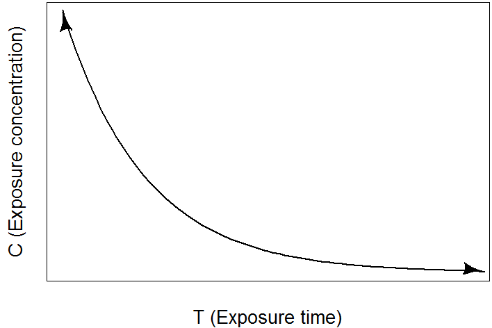
For adaptive construction management, this may not be sufficient, as operations are time-dependent and operational decisions need to be made at short notice. Another issue to be considered is therefore the factor ‘time’. First of all, in toxicology, SSDs are based on chronic end-points, which is actually a worst-case approach. The idea behind this is that if a species is not affected after chronic exposure, it will certainly not be affected after a shorter exposure. Unfortunately, examples of time-dependent SSDs are scarce in literature. In fact, there is only one publication (Smit et al., 2008c) in which a time-dependent SSD (for hydrogen peroxide exposure) is actually developed. In this approach, several constant concentrations were tested, and effects on several species were recorded as a function of time. This gives a simple and straightforward relationship between exposure time and effect, known as Habers’ Law (Karman, 2000). To achieve the same effect with higher exposure concentrations, a shorter exposure duration is required and vice versa. Note that this relationship applies to constant stress levels and is not suitable for fluctuating exposure levels.
For toxicants models are available that can describe effects of fluctuating exposure concentrations. For example, some models consider the kinetics (uptake and excretion speeds) of toxicants. With such kinetic information, internal concentration in a species can be calculated from a (fluctuating) external concentration. This internal concentration can then be compared with internal effect threshold levels, in order to determine effects as a function of time (see for example Figure, Graphical representation of inverse hazard model, applied to three hypothetical cases, ref Karman, 2000). A similar, more mechanistic approach (e.g., considering uptake, storage and excretion processes and target sites in the organism) would also be possible for non-toxic stressors (such as suspended matter), although this requires knowledge on the mechanism through which these stressors affect the organism, as well as data to quantify them.
Although the latter approach (figure c) accounts for the factor ‘time’ in a more realistic and sophisticated way, it doesn’t take the recovery potential of a species into account. Furthermore, it is difficult to implement this approach in a simple SSD approach, as effects will not only depend on the exposure time and the current exposure level, but also on the exposure history.
As these examples illustrate, including spatial and temporal effects complicate the SSD methodology. Therefore, it is advisable to start with a simple approach, viz. a generic SSD based on worst-case end-points (e.g. chronic NOECs) and to add data and realism (hence complexity) only when required. This is actually the approach implemented by the Norwegian offshore oil and gas industry as described under Practical Applications section.
4. Conclusions and recommendations
SSDs can be applied:
- to identify and rank the substances by their contribution to the overall probability of affecting sensitive species;
- to select, on an environmental cost/benefit basis, (potential) discharge reducing measures (BAT/BEP techniques, see Practical Applications section for more details);
- to compare the environmental risks of different projects/operational strategies;
- to serve as basis for environmental monitoring.
A comparison with effect data for other types of suspended particulate matter should indicate the general applicability of the derived SSDs for activities other than offshore oil and gas drilling. The fate of the sediment particles during and after marine construction activities should be modeled. Available exposure models should be identified.